深度学习神经网络特征提取(三)
MobileNet简介
在之前的文章中已经介绍了VGG和ResNet相关的网络结构,随着深度学习的发展,都在追求精度和准确性,因此也导致了网络层数的加深抑或网络的扩展。然而随着网络的不断加深和扩展,参数的数量也在急剧上升,从而导致性能的下降。MobileNet的出现也正是为了解决这种情况。
MobileNetv1
MobileNetv1网络特点主要集中于提出的深度可分离卷积,其网络结构部分只是线性连接,如下图所示。

深度可分离卷积
介绍深度可分离卷积,那我们不得不与常规的卷积进行对比,常规的卷积操作如下图。
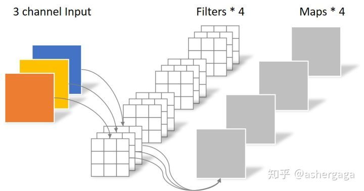
对于一张通道数为3,长宽为5的输入图像,经过3x3的卷积核,且输出层数为4的卷积时,其卷积核的真实情况如上图,在此种情况下参数量为:4x3x3x3=108。
而在深度可分离卷积中,我们进行同样的3x3的卷积核,且输出层数为4的卷积时,其操作情况如下两张图片。
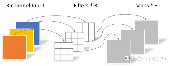
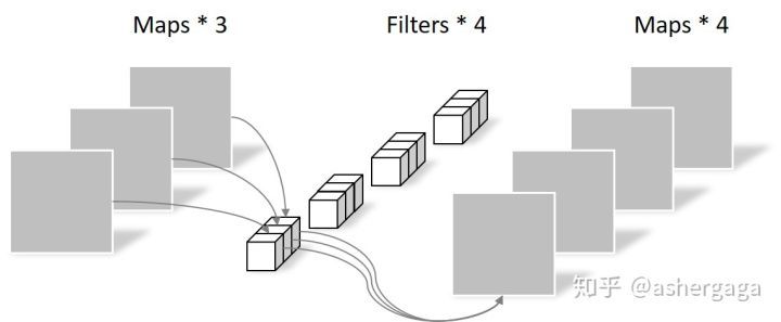
在深度可分离卷积中,首先通过N个3x3的卷积核(其中N为输入的层数,在图一中N为3)与输入层数一一对应进行特征提取,然后再通过M个1xN的卷积进行层数的缩放(图2)。在这种情况下,参数量为:3x3x3+1x1x3x4=39。相较于常规卷积操作,深度可分离卷积的参数量下降了很多,大大提高了模型的运行性能,并且对最终的结果的精确度影响并不是很高。
MobileNetv1的网络结构
在上图中,我们给出了MobileNetv1的网络结构,主要处理流程为:
- (步长为2的卷积和归一化)x 1
- (步长为1的深度可分离卷积和归一化,步长为1的卷积和归一化,步长为2的深度可分离卷积和归一化,步长为1的卷积和归一化)x 3
- (步长为1的深度可分离卷积和归一化,步长为1的卷积和归一化)x 5
- (步长为2的深度可分离卷积和归一化,步长为1的卷积和归一化)x 2
- 一次7x7平均池化,一层全连接层
- 最后softmax层
代码如下:
#-------------------------------------------------------------#
#   MobileNet的网络部分
#-------------------------------------------------------------#
def MobileNet(input_shape=[224,224,3], depth_multiplier=1, dropout=1e-3, classes=1000):
    img_input = Input(shape=input_shape)

    # 224,224,3 -> 112,112,32
    x = _conv_block(img_input, 32, strides=(2, 2))

    # 112,112,32 -> 112,112,64
    x = _depthwise_conv_block(x, 64, depth_multiplier, block_id=1)

    # 112,112,64 -> 56,56,128
    x = _depthwise_conv_block(x, 128, depth_multiplier, strides=(2, 2), block_id=2)
    # 56,56,128 -> 56,56,128
    x = _depthwise_conv_block(x, 128, depth_multiplier, block_id=3)

    # 56,56,128 -> 28,28,256
    x = _depthwise_conv_block(x, 256, depth_multiplier, strides=(2, 2), block_id=4)

    # 28,28,256 -> 28,28,256
    x = _depthwise_conv_block(x, 256, depth_multiplier, block_id=5)

    # 28,28,256 -> 14,14,512
    x = _depthwise_conv_block(x, 512, depth_multiplier, strides=(2, 2), block_id=6)

    # 14,14,512 -> 14,14,512
    x = _depthwise_conv_block(x, 512, depth_multiplier, block_id=7)
    x = _depthwise_conv_block(x, 512, depth_multiplier, block_id=8)
    x = _depthwise_conv_block(x, 512, depth_multiplier, block_id=9)
    x = _depthwise_conv_block(x, 512, depth_multiplier, block_id=10)
    x = _depthwise_conv_block(x, 512, depth_multiplier, block_id=11)

    # 14,14,512 -> 7,7,1024
    x = _depthwise_conv_block(x, 1024, depth_multiplier, strides=(2, 2), block_id=12)
    x = _depthwise_conv_block(x, 1024, depth_multiplier, block_id=13)

    # 7,7,1024 -> 1,1,1024
    x = GlobalAveragePooling2D()(x)
    x = Reshape((1, 1, 1024), name='reshape_1')(x)
    x = Dropout(dropout, name='dropout')(x)
    x = Conv2D(classes, (1, 1),padding='same', name='conv_preds')(x)
    x = Activation('softmax', name='act_softmax')(x)
    x = Reshape((classes,), name='reshape_2')(x)

    inputs = img_input

    model = Model(inputs, x, name='mobilenet_1_0_224_tf')
    return model

def _conv_block(inputs, filters, kernel=(3, 3), strides=(1, 1)):
    x = Conv2D(filters, kernel, padding='same', use_bias=False, strides=strides, name='conv1')(inputs)
    x = BatchNormalization(name='conv1_bn')(x)
    return Activation(relu6, name='conv1_relu')(x)


def _depthwise_conv_block(inputs, pointwise_conv_filters, depth_multiplier=1, strides=(1, 1), block_id=1):

    x = DepthwiseConv2D((3, 3), padding='same', depth_multiplier=depth_multiplier, strides=strides, use_bias=False, name='conv_dw_%d' % block_id)(inputs)

    x = BatchNormalization(name='conv_dw_%d_bn' % block_id)(x)
    x = Activation(relu6, name='conv_dw_%d_relu' % block_id)(x)

    x = Conv2D(pointwise_conv_filters, (1, 1), padding='same', use_bias=False, strides=(1, 1), name='conv_pw_%d' % block_id)(x)
    x = BatchNormalization(name='conv_pw_%d_bn' % block_id)(x)
    return Activation(relu6, name='conv_pw_%d_relu' % block_id)(x)

def relu6(x):
    return K.relu(x, max_value=6)
MobileNetv2
MobileNetv2网络特点相较于MobileNetv1提出了反残差结构和线性瓶颈结构,总体网络结构如下图所示。
反残差结构和线性瓶颈结构
反残差结构是相对于ResNet50而言的,此外MobileNetv2的基础结构和ResNet的基础结构一样,同样是双分支残差连接:
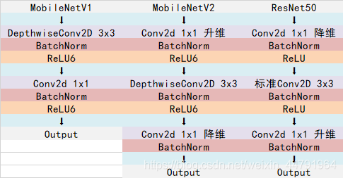
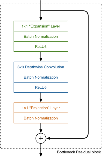
其中ResNet50中先卷积降维,然后进行3x3卷积提取特征,然后在进行升维,这样做在实际中部证明是比直接3x3卷积效果更好的。而在MobileNetv2中,反向进行操作。
而所谓的线性瓶颈结构则是在卷积降维之后不再进行ReLu6层激活,保证提取得到的特征不被破坏,直接与输入相加。
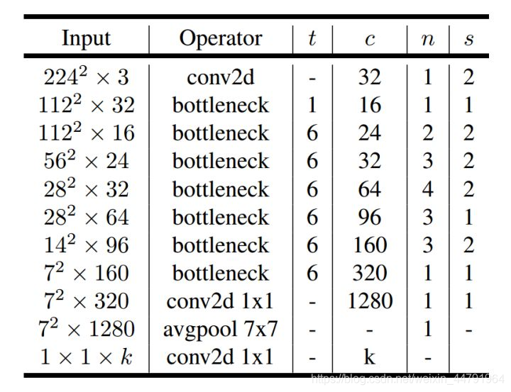
MobileNetv2的网络结构
在上图中,我们给出了MobileNetv2的网络结构,主要处理流程为:
- 步长为2的卷积层 x 1
- 步长为1的瓶颈层 x 1
- 步长为2的瓶颈层 x 3
- 步长为1的瓶颈层 x 1
- 步长为2的瓶颈层 x 1
- 步长为1的瓶颈层 x 1
- 步长为1的卷积层 x 1
- 7x7 平均池化层 x 1
- 全连接层softmax分类
代码如下:
#-------------------------------------------------------------#
#   MobileNetV2的网络部分
#-------------------------------------------------------------#
# relu6!
def relu6(x):
    return K.relu(x, max_value=6)


def MobileNetV2(input_shape=[224,224,3], classes=1000):

    img_input = Input(shape=input_shape)

    # 224,224,3 -> 112,112,32
    x = ZeroPadding2D(padding=(1, 1), name='Conv1_pad')(img_input)
    x = Conv2D(32, kernel_size=3, strides=(2, 2), padding='valid', use_bias=False, name='Conv1')(x)
    x = BatchNormalization(epsilon=1e-3, momentum=0.999, name='bn_Conv1')(x)
    x = Activation(relu6, name='Conv1_relu')(x)

    # 112,112,32 -> 112,112,16
    x = _inverted_res_block(x, filters=16, stride=1,expansion=1, block_id=0)

    # 112,112,16 -> 56,56,24
    x = _inverted_res_block(x, filters=24, stride=2, expansion=6, block_id=1)
    x = _inverted_res_block(x, filters=24, stride=1, expansion=6, block_id=2)

    # 56,56,24 -> 28,28,32
    x = _inverted_res_block(x, filters=32, stride=2, expansion=6, block_id=3)
    x = _inverted_res_block(x, filters=32, stride=1, expansion=6, block_id=4)
    x = _inverted_res_block(x, filters=32, stride=1, expansion=6, block_id=5)

    # 28,28,32 -> 14,14,64
    x = _inverted_res_block(x, filters=64, stride=2, expansion=6, block_id=6)
    x = _inverted_res_block(x, filters=64, stride=1, expansion=6, block_id=7)
    x = _inverted_res_block(x, filters=64, stride=1, expansion=6, block_id=8)
    x = _inverted_res_block(x, filters=64, stride=1, expansion=6, block_id=9)

    # 14,14,64 -> 14,14,96
    x = _inverted_res_block(x, filters=96, stride=1, expansion=6, block_id=10)
    x = _inverted_res_block(x, filters=96, stride=1, expansion=6, block_id=11)
    x = _inverted_res_block(x, filters=96, stride=1, expansion=6, block_id=12)
    # 14,14,96 -> 7,7,160
    x = _inverted_res_block(x, filters=160, stride=2, expansion=6, block_id=13)
    x = _inverted_res_block(x, filters=160, stride=1, expansion=6, block_id=14)
    x = _inverted_res_block(x, filters=160, stride=1, expansion=6, block_id=15)

    # 7,7,160 -> 7,7,320
    x = _inverted_res_block(x, filters=320, stride=1, expansion=6, block_id=16)

    # 7,7,320 -> 7,7,1280
    x = Conv2D(1280, kernel_size=1, use_bias=False, name='Conv_1')(x)
    x = BatchNormalization(epsilon=1e-3, momentum=0.999, name='Conv_1_bn')(x)
    x = Activation(relu6, name='out_relu')(x)

    x = GlobalAveragePooling2D()(x)
    x = Dense(classes, activation='softmax', use_bias=True, name='Logits')(x)

    inputs = img_input

    model = Model(inputs, x)

    return model


def _inverted_res_block(inputs, expansion, stride, pointwise_filters, block_id):
    in_channels = backend.int_shape(inputs)[-1]
    x = inputs
    prefix = 'block_{}_'.format(block_id)

    # part1 数据扩张
    if block_id:
        # Expand
        x = Conv2D(expansion * in_channels, kernel_size=1, padding='same', use_bias=False, activation=None, name=prefix + 'expand')(x)
        x = BatchNormalization(epsilon=1e-3, momentum=0.999, name=prefix + 'expand_BN')(x)
        x = Activation(relu6, name=prefix + 'expand_relu')(x)
    else:
        prefix = 'expanded_conv_'

    if stride == 2:
        x = ZeroPadding2D(padding=(1,1), name=prefix + 'pad')(x)

    # part2 可分离卷积
    x = DepthwiseConv2D(kernel_size=3, strides=stride, activation=None, use_bias=False, padding='same' if stride == 1 else 'valid', name=prefix + 'depthwise')(x)
    x = BatchNormalization(epsilon=1e-3, momentum=0.999, name=prefix + 'depthwise_BN')(x)

    x = Activation(relu6, name=prefix + 'depthwise_relu')(x)

    # part3压缩特征,而且不使用relu函数,保证特征不被破坏
    x = Conv2D(pointwise_filters, kernel_size=1, padding='same', use_bias=False, activation=None, name=prefix + 'project')(x)

    x = BatchNormalization(epsilon=1e-3, momentum=0.999, name=prefix + 'project_BN')(x)

    if in_channels == pointwise_filters and stride == 1:
        return Add(name=prefix + 'add')([inputs, x])
    return x
MobileNetv3
MobileNetv3网络特点相较于MobileNetv2主要添加了以下特点:
- 轻量级的注意力机制
- 利用h-swish代替swish函数
主要网络结构有两种,一种large,一种small,主要区别在于通道数和基础块的次数,本文介绍small类型,网络结构如下:
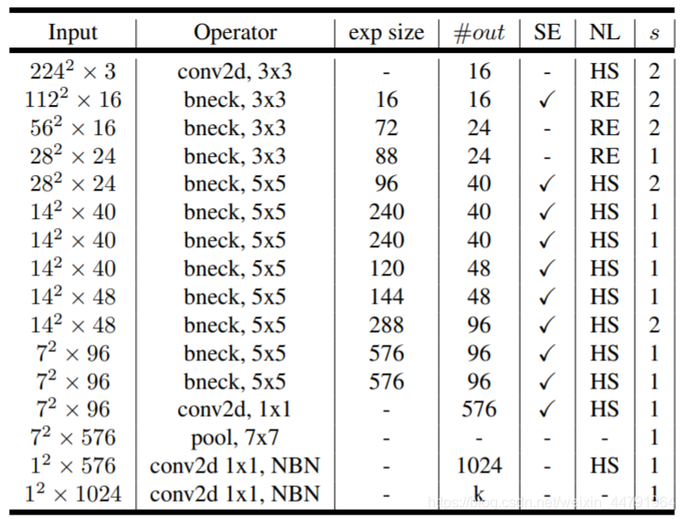
轻量级注意力机制引入
在MobileNetv3中,由于轻量级注意力机制的引入,使得原来的基础块结构产生了一些变化,新的结构如图所示:

从上图我们可以直观的感受到,轻量级注意力机制的引入主要用于改变各个特征层之间的权重系数。
相信通过前面代码的学习你对特征提取的网络已经有了一定的了解,那么下面的代码就很容易理解了。
代码如下:
alpha = 1
def relu6(x):
    # relu函数
    return K.relu(x, max_value=6.0)

def hard_swish(x):
    # 利用relu函数乘上x模拟sigmoid
    return x * K.relu(x + 3.0, max_value=6.0) / 6.0

def return_activation(x, nl):
    # 用于判断使用哪个激活函数
    if nl == 'HS':
        x = Activation(hard_swish)(x)
    if nl == 'RE':
        x = Activation(relu6)(x)

    return x

def conv_block(inputs, filters, kernel, strides, nl):
    # 一个卷积单元,也就是conv2d + batchnormalization + activation
    channel_axis = 1 if K.image_data_format() == 'channels_first' else -1

    x = Conv2D(filters, kernel, padding='same', strides=strides)(inputs)
    x = BatchNormalization(axis=channel_axis)(x)

    return return_activation(x, nl)

def squeeze(inputs):
    # 注意力机制单元
    input_channels = int(inputs.shape[-1])

    x = GlobalAveragePooling2D()(inputs)
    x = Dense(int(input_channels/4))(x)
    x = Activation(relu6)(x)
    x = Dense(input_channels)(x)
    x = Activation(hard_swish)(x)
    x = Reshape((1, 1, input_channels))(x)
    x = Multiply()([inputs, x])

    return x

def bottleneck(inputs, filters, kernel, up_dim, stride, sq, nl):
    channel_axis = 1 if K.image_data_format() == 'channels_first' else -1

    input_shape = K.int_shape(inputs)

    tchannel = int(up_dim)
    cchannel = int(alpha * filters)

    r = stride == 1 and input_shape[3] == filters
    # 1x1卷积调整通道数,通道数上升
    x = conv_block(inputs, tchannel, (1, 1), (1, 1), nl)
    # 进行3x3深度可分离卷积
    x = DepthwiseConv2D(kernel, strides=(stride, stride), depth_multiplier=1, padding='same')(x)
    x = BatchNormalization(axis=channel_axis)(x)
    x = return_activation(x, nl)
    # 引入注意力机制
    if sq:
        x = squeeze(x)
    # 下降通道数
    x = Conv2D(cchannel, (1, 1), strides=(1, 1), padding='same')(x)
    x = BatchNormalization(axis=channel_axis)(x)


    if r:
        x = Add()([x, inputs])

    return x

def MobileNetv3_small(shape = (224,224,3),n_class = 1000):
    inputs = Input(shape)
    # 224,224,3 -> 112,112,16
    x = conv_block(inputs, 16, (3, 3), strides=(2, 2), nl='HS')

    # 112,112,16 -> 56,56,16
    x = bottleneck(x, 16, (3, 3), up_dim=16, stride=2, sq=True, nl='RE')

    # 56,56,16 -> 28,28,24
    x = bottleneck(x, 24, (3, 3), up_dim=72, stride=2, sq=False, nl='RE')
    x = bottleneck(x, 24, (3, 3), up_dim=88, stride=1, sq=False, nl='RE')

    # 28,28,24 -> 14,14,40
    x = bottleneck(x, 40, (5, 5), up_dim=96, stride=2, sq=True, nl='HS')
    x = bottleneck(x, 40, (5, 5), up_dim=240, stride=1, sq=True, nl='HS')
    x = bottleneck(x, 40, (5, 5), up_dim=240, stride=1, sq=True, nl='HS')
    # 14,14,40 -> 14,14,48
    x = bottleneck(x, 48, (5, 5), up_dim=120, stride=1, sq=True, nl='HS')
    x = bottleneck(x, 48, (5, 5), up_dim=144, stride=1, sq=True, nl='HS')

    # 14,14,48 -> 7,7,96
    x = bottleneck(x, 96, (5, 5), up_dim=288, stride=2, sq=True, nl='HS')
    x = bottleneck(x, 96, (5, 5), up_dim=576, stride=1, sq=True, nl='HS')
    x = bottleneck(x, 96, (5, 5), up_dim=576, stride=1, sq=True, nl='HS')

    x = conv_block(x, 576, (1, 1), strides=(1, 1), nl='HS')
    x = GlobalAveragePooling2D()(x)
    x = Reshape((1, 1, 576))(x)

    x = Conv2D(1024, (1, 1), padding='same')(x)
    x = return_activation(x, 'HS')

    x = Conv2D(n_class, (1, 1), padding='same', activation='softmax')(x)
    x = Reshape((n_class,))(x)

    model = Model(inputs, x)

    return model